Next: B..2.1.2 solve_ivp() の利用 Up: B..2.1 Malthus モデル Previous: B..2.1 Malthus モデル
詳しいことは scipy.integrate.odeint -- ScyPy 1.11.3 Manual を見よ。
微分方程式 (B.1a) の右辺に現れる ![]() を計算する関数 func を作れば、簡単に解が求まる。
を計算する関数 func を作れば、簡単に解が求まる。
次のプログラムでは、malthus() というのが
![]() を計算する関数である。
を計算する関数である。
![]() という簡単な関数なので、実質2行だけである。
という簡単な関数なので、実質2行だけである。
| malthus1.py |
# malthus1.py --- dx/dt=a*x, x(0)=x0 を解いて解曲線を描く
import numpy as np
from scipy.integrate import odeint
import matplotlib.pyplot as plt
def malthus(x, t, a): # f(x,t,パラメーター)
return a * x
a=1
t0=0; T=1; n=10
t=np.linspace(t0,T,n+1)
x0=1
sol=odeint(malthus, x0, t, args=(a,)) # 解を求める
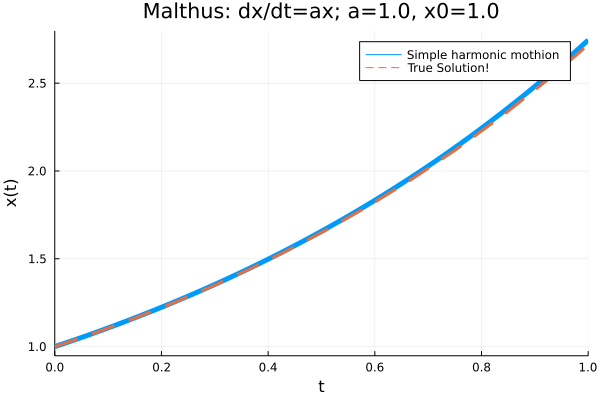
plt.plot(t,sol) # 解曲線描画
plt.ylim(0, 3) # 縦軸の範囲指定
# タイトル、凡例の位置、横軸と縦軸の説明、グリッド
plt.title('Malthus: dx/dt=ax, x(0)=x0; a='+str(a)+', x0='+str(x0))
plt.xlabel('t')
plt.ylabel('x')
plt.grid()
plt.show()
|
次の2行で、区間 ![]() の10等分点を計算して、
変数 t に記憶している。
の10等分点を計算して、
変数 t に記憶している。
t0=0; T=1; n=10 t=np.linespace(t0,T,n+1) |
sol=odeint(malthus, x0, t, arg=(a,)) で解を計算している。
![]() というのは見慣れない書き方かもしれないが、
a をオプションのパラメーターとして渡す仕組みを使っている
(パラメーターが1個のときは最後に , をつける必要があるらしい)。
というのは見慣れない書き方かもしれないが、
a をオプションのパラメーターとして渡す仕組みを使っている
(パラメーターが1個のときは最後に , をつける必要があるらしい)。
この後、解をどのように出力するかは、色々なやり方がある。 ここでは matplotlib.pyplot の plot() を用いて 解のグラフ (解曲線) を描いている (グラフ描きは、微分方程式とは直接関係ないので、 多くの Python の入門書に説明が書いてある。)。
では次に複数の解の様子を同時に眺めてみる。 初期値を変えて解を求めて、その解曲線を描き足していく。
| malthus2.py |
# malthus2.py --- dx/dt=a*x, x(0)=x0 を複数の初期値について解いて解曲線を描く

import numpy as np
from scipy.integrate import odeint
import matplotlib.pyplot as plt

def malthus(x, t, a):
    return a * x

a=1
t0=0; T=1; n=10
t=np.linspace(t0,T,n+1)

for i in range(0,10):
    x0=i*0.2
    sol=odeint(malthus, x0, t, args=(a,))
    plt.plot(t,sol)
    # 解曲線描画
    plt.plot(t,sol, label='x0='+'{:6.1f}'.format(x0))

plt.ylim(0, 5)  # 縦軸の範囲指定

# タイトル、凡例の位置、横軸と縦軸の説明、グリッド
plt.title('Malthus: dx/dt=ax, x(0)=x0; a='+str(a))
plt.legend(loc='upper left')
plt.xlabel('t')
plt.ylabel('x')
plt.grid()

plt.show()
|
当たり前のことであるが、解の一意性が成り立つので、解曲線は互いに交わらない。
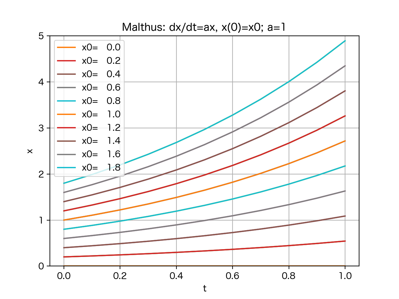 (コピーするとモノクロになって分かりにくいけれど…)