2.1 Dirichlet境界値問題

$$-u''(x)=f(x)$$   ( $x\in (0,L)$)$$,\quad u(0)=u(L)=0$$

$$h=\frac{L}{N},\quad x_i=ih$$   ( $i=0,1,\cdots,N$)$$.$$

$$\frac{1}{h^2} \begin{pmatrix} 2 & -1 \\ -1 & 2 & -1 \\ & -1... ...begin{pmatrix} f(x_1) \\ f(x_2) \\ \vdots \\ f(x_{N-1}) \end{pmatrix}.$$

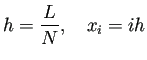laplacian1d.m

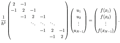
% laplacian1d.m
% curl -O https://m-katsurada.sakura.ne.jp/program/fdm/laplacian1d.m
% -(d/dx)^2 の差分近似
% [0,L] を N 等分した時の行列は h=L/N; a=laplacian1d(N-1)/(h*h);
function a=laplacian1d(m)
  e=ones(m,1);
  a=spdiags([-e 2*e -e],-1:1,m,m); % 疎行列なので圧縮した形式
end

>> a=laplacian1d(3));
>> full(a)

ans =
     2    -1     0
    -1     2    -1
     0    -1     2

$I=(0,L)$ を $N$ 等分する差分近似の場合は

>> L=1;
>> n=5;
>> h=L/n;
>> a=laplacian1d(n-1)/(h*h);
>> full(a)

ans =

   50.0000  -25.0000         0         0
  -25.0000   50.0000  -25.0000         0
         0  -25.0000   50.0000  -25.0000
         0         0  -25.0000   50.0000

$I=(0,L)$ における

$$-u''(x)=1,\quad u(0)=u(L)=0$$

を解くには ($f\equiv 1$ とするのは安直だけど)

poisson1d_test1.m

L=1
n=10
h=L/n
x=linspace(0,L,n+1);
a=laplacian1d(n-1)/(h*h);
f=ones(n-1,1);
u=a\f;
u=[0; u; 0];
plot(x,u)
figure(gcf)

とする。

$f(x)=\sin x$ の場合は

poisson1d_test2.m

L=1
n=10
h=L/n
x=linspace(0,L,n+1);
a=laplacian1d(n-1)/(h*h);
f=sin(x(2:n))';
u=a\f;
u=[0; u; 0];
plot(x,u)
figure(gcf)

とする。

$f(x)=x(1-x)$ の場合は

poisson1d_test3.m

L=1
n=10
h=L/n
x=linspace(0,L,n+1);
a=laplacian1d(n-1)/(h*h);
f=x.*(1-x);
f=f(2:n)';
u=a\f;
u=[0; u; 0];
plot(x,u)
figure(gcf)

とする。

(2024/9 改訂版) 非同次Dirichlet境界値問題のプログラム。

poisson1d_nh.m

% poisson1d_nh.m
% 1次元領域におけるPoisson -△u=f (非同次Dirichlet境界条件) を差分法で解く
% 入手 curl -O https://m-katsurada.sakura.ne.jp/program/fdm/poisson1d_nh.m
% 解説 https://m-katsurada.sakura.ne.jp/labo/text/poisson1d.pdf
% (2024/9/4)。
function poisson1d_nh(N)
  arguments
    N=4 % デバッグ用
  end
  function K = poisson1d_mat(W,N)
    h=W/N;
    I=speye(N-1,N-1);
    v=ones(N-2,1);
    J=sparse(diag(v,1)+diag(v,-1));
    K=2*I-J;
    K=1/h^2*K;
  end
  % 想定している厳密解
  function val = exact_solution(x)% =x^4
    val = x .^ 4;
    %val = (x - 1.0/2).^2;
  end
  % f=-△u=-d^2u/dx^2
  function val = f(x)% = -u''(x) = -12x^2
    val = - 12 * x.^2;
    %val = 0 .* x - 2.0;
  end
  % 領域
  a=0; b=1;
  % 境界値
  alpha = exact_solution(a);
  beta = exact_solution(b);
  fprintf('a=%f, b=%f, u(a)=%f, u(b)=%f\n', a, b, alpha, beta);
  % 差分近似の行列
  h=(b-a)/N;
  fprintf('N=%d, h=%g\n', N, h);
  A=poisson1d_mat(b-a,N);
  if N <= 10
    disp('A='); disp(full(A));
  end
  % 連立方程式の右辺
  X=linspace(a,b,N+1);
  F=f(X(2:N)');
  F(1)=F(1)+alpha/h^2;
  F(N-1)=F(N-1)+beta/h^2;
  if N <= 10
    disp('X='); disp(X);
    disp('F=f(X)='); disp(F');
  end
  % 差分解を求める
  u=zeros(N+1,1);
  u(2:N)=A\F;
  % 境界値
  u(1)=alpha; u(N+1)=beta;
  % グラフを描く
  plot(X,u); title('差分解のグラフ'); drawnow; shg;
  figure
  plot(X,exact_solution(X')); title('厳密解のグラフ'); drawnow; shg;
  exact=exact_solution(X');
  error=norm(u-exact,inf);
  fprintf('max norm of error=%e\n', error);
end

入手するにはターミナルで

curl -O https://m-katsurada.sakura.ne.jp/program/fdm/poisson1d_nh.m

これを実行するには、例えば

cp -p poisson1d_nh.m ~/Documents/MATLAB

とコピーして (私はシンボリック・リンクをはることにしている)、 MATLAB の中で

>> poisson1d_nh

(分割数はデフォールトの $N=4$ が採用される。)

あるいは、分割数 $N$ を指定するため

>> poisson1d_nh(10)

のようにする。

上のサンプル・プログラムでは、 $u(x)=x^4$ と選び、 $f(x)=-u''(x)=-12x^2$, $\alpha=u(0)=0$, $\beta=u(1)=1$ としてある。 $N$ を $10$ から倍々にしていくと以下のようになった。

N=10, h=0.1
max norm of error=2.500000e-03

N=20, h=0.05
max norm of error=6.250000e-04

N=40, h=0.025
max norm of error=1.562500e-04

N=80, h=0.0125
max norm of error=3.906250e-05

N=160, h=0.00625
max norm of error=9.765625e-06

N=320, h=0.003125
max norm of error=2.441406e-06

$N$が$2$倍になると誤差は $\frac{1}{4}$ 倍になる。 誤差は $O(1/N^2)$ になっているようで、ひとまずは納得できる。